The mental model: what a language model actually is
I.1 Next-token prediction is the whole game
A language model (LM) is a function that takes a sequence of text and outputs a probability for every possible next piece of text. That's it. "The cat sat on the ___" → {mat: 9%, floor: 7%, couch: 5%, ...}. Generation is just running this in a loop: predict, pick, append, repeat.
Everything impressive an LLM (Large Language Model, same thing, but big) does, code, reasoning, tool calls, is an emergent consequence of getting extremely good at this one prediction task over an enormous amount of text. Training is the process of getting good at it.
I.2 Tokens: the model's alphabet
Models don't read characters or words, they read tokens, chunks produced by a tokenizer. A token is usually 3–5 characters (~¾ of an English word). "unbelievable" might be un|believ|able. The tokenizer is built once (before pretraining) with an algorithm called BPE (Byte-Pair Encoding): start with single bytes, repeatedly merge the most frequent adjacent pair, stop at a target vocabulary size (typically 32k–256k entries).
Why you care:
- Context windows are measured in tokens (Kimi's 131k context ≈ a 300-page book).
- Datasets are measured in tokens (pretraining runs consume trillions).
- Speed is measured in tokens/second (your Kimi does ~15 tok/s decode).
- Weird model behaviors (bad at counting letters, arithmetic quirks) are often tokenizer artifacts.
I.3 Parameters, weights, and what "8B" means
A model is a giant pile of numbers called parameters or weights (the terms are interchangeable). "Llama-3.2-3B" = 3 billion parameters. Each is a small number (like 0.0231 or -1.7) that gets multiplied against inputs as data flows through the network. Training = adjusting these numbers. A trained model file is literally just these numbers serialized to disk, which is why an 8B model in bf16 (2 bytes per parameter, see Part II.4) is a ~16 GB download.
I.4 The transformer, at cocktail-party depth
Every modern LLM is a transformer, an architecture from the 2017 paper Attention Is All You Need. You don't need the math, but the vocabulary shows up everywhere, so here's the tour:
- Embedding: the lookup table that turns each token into a vector (a list of ~2,000–16,000 numbers) the network can process.
- Attention: the mechanism that lets each token "look at" every previous token and decide which ones matter for predicting what comes next. This is the magic ingredient, it's how the model connects "her" back to "Alice" from three paragraphs ago.
- Attention heads: attention runs many times in parallel with different learned "perspectives"; each parallel copy is a head. MHA (Multi-Head Attention) is the vanilla version; GQA (Grouped-Query Attention) and MLA (Multi-head Latent Attention, what Kimi/DeepSeek use, you've seen
TRITON_MLAin the vLLM logs) are memory-saving refinements. - FFN / MLP (Feed-Forward Network / Multi-Layer Perceptron): the other half of each layer, a plain "multiply by big matrices" block where most of the parameters live.
- Layers / blocks: one attention + one FFN = a block; models stack 24–100+ of them.
- KV cache (Key-Value cache): during generation, the model caches per-token attention data so it doesn't recompute the whole history for every new token. This is what eats your serving memory, vLLM's "KV cache: 763,840 tokens" log line is this.
- MoE (Mixture of Experts): instead of one FFN per layer, have many ("experts") and route each token to a few of them. You get a huge parameter count with modest compute per token, Kimi K2.6 is 519B parameters total but only activates ~30B per token. This is why it's fast enough on your Sparks. Dense models (Llama, Qwen-dense) activate everything, always.
Only active weights are streamed per token, so decode speed scales with the 30B, while capacity scales with the 519B.
Your hardware, demystified
II.1 What a GB10 actually is
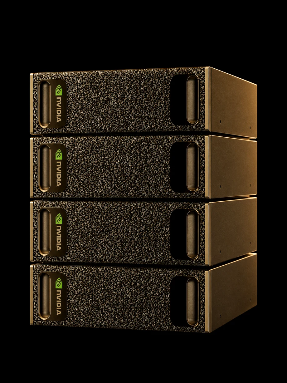
Each DGX Spark contains one GB10 Grace-Blackwell Superchip:
- Grace = the CPU side: 20 ARM cores (aarch64 architecture, this is why x86 binaries don't run and why some Python wheels need special builds).
- Blackwell = the GPU side: NVIDIA's 2024+ GPU generation (successor to Hopper/H100 and Ada/RTX-40).
- Unified memory: 128 GB of LPDDR5X shared by CPU and GPU. On a normal PC, the GPU has its own small fast VRAM (say 24 GB GDDR) and copying data across the PCIe bus is slow and explicit. Here, there is one pool; the GPU can touch all 128 GB. This is the estate's superpower, models that OOM (Out Of Memory) on a 24 GB RTX card just… fit.
II.2 The two currencies: FLOPs and bandwidth
Two numbers govern everything in ML hardware:
- FLOPs (Floating-Point Operations per Second): raw math speed. The GB10 does ~1 PFLOP (petaFLOP = 10¹⁵) of sparse FP4, a huge number.
- Memory bandwidth: how fast weights can be streamed from memory to the compute units. The GB10 does 273 GB/s.
Here's the insight that explains all of your benchmarking results: for LLM work, bandwidth is usually the bottleneck, not FLOPs. To generate one token, the model must read every active weight once. Kimi's ~30B active params in 4-bit ≈ 15 GB per token per node → 273/15 ≈ 18 tokens/s theoretical → you measured 15. The math checks out; the GPU's compute units spend most of their time waiting for memory.
Training has the same character but reads and writes far more data per step (weights + gradients + optimizer state, see Part V.1). A datacenter H100 has 3,350 GB/s, 12× your bandwidth, which is why we're not pretraining Llama here. But for LoRA finetunes of small-to-mid models, 273 GB/s is entirely serviceable.
(30B active × 0.5 B/param)
273 GB/s ÷ 15 GB
the math checks out
Same measure, ordered magnitude → one amber ramp. The compute units mostly wait on memory.
II.3 sm_121, CUDA, and why you've been patching kernels
- CUDA (Compute Unified Device Architecture): NVIDIA's programming platform for GPUs. Everything, PyTorch, vLLM, our training, compiles down to CUDA.
- Compute capability / sm_XX: each GPU generation has a version number ("sm" = streaming multiprocessor). H100 = sm_90, RTX 5090 = sm_120, GB10 = sm_121. Libraries ship pre-compiled kernels per sm; sm_121 is new and niche enough that you've already lived the consequences, the Triton shared-memory patch and the DeepGEMM sm_121 blocker from the Kimi/GLM saga were both "nobody compiled for this chip yet" problems. Expect one or two of the same in training-land (bitsandbytes, flash-attention), which is why validating the stack is Stage 0 of the curriculum.
- Kernel: a small GPU program (e.g., "multiply these matrices"). Triton is a Python-like language for writing them (used heavily inside vLLM and PyTorch).
II.4 Precision formats: FP32 → NVFP4
Numbers can be stored at different precisions; less precision = smaller + faster (less bandwidth!) at some accuracy cost. The zoo:
| Format | Bytes/param | Role |
|---|---|---|
| FP32 (single precision) | 4 | Classic default; today only optimizer internals |
| TF32 | ~2.4 effective | NVIDIA's FP32-lite for matmuls; automatic |
| FP16 (half) | 2 | Older mixed-precision; can overflow (numeric range too small) |
| BF16 (bfloat16, "brain float") | 2 | The training standard. Same range as FP32, less precision, stable and fast |
| FP8 | 1 | Serving + cutting-edge training; your KV caches run fp8 |
| FP4 / NVFP4 | 0.5 | 4-bit; NVFP4 is NVIDIA's block-scaled variant, every model you serve (Kimi, GLM, V4-Flash) is NVFP4-quantized |
| INT8/INT4 | 1 / 0.5 | Integer quantization (GPTQ/AWQ world, see Part VI) |
| NF4 (NormalFloat-4) | 0.5 | 4-bit format designed for QLoRA finetuning (Part V.4) |
Mixed precision = train with bf16 weights/activations but keep a master FP32 copy inside the optimizer for stability. Frameworks do this automatically; you'll just see bf16=True in configs.
One hue, light→dark with magnitude. An 8B model is a 32 GB download in FP32 and a 4 GB one in NVFP4.
II.5 The fabric: how 4 Sparks become one machine
- ConnectX-7: the 200 Gb/s NICs (Network Interface Cards) in each Spark.
- RoCE (RDMA over Converged Ethernet): lets one machine read/write another's memory directly (RDMA = Remote Direct Memory Access) without bothering the CPU, this is the
rocep1s0f1interface in your launch scripts. - NCCL (NVIDIA Collective Communications Library, "nickel"): the library every distributed job uses to move tensors between GPUs, same NCCL whether it's vLLM tensor-parallel serving or our future FSDP training. The "collectives" are named operations: all-reduce (everyone averages their copies, the heartbeat of data-parallel training), all-gather, broadcast, reduce-scatter.
- 200 Gb/s ≈ 25 GB/s ≈ 1/11th of local memory bandwidth. Rule of thumb: the fabric is fine for exchanging gradients (DDP) and shards (FSDP), painful for anything chattier, one reason multi-node graph capture never worked for GLM.
The training loop, for real this time
This is the part to actually internalize. Every training framework, from nanoGPT's 300 lines to a trillion-parameter lab run, is this loop:
for each batch of examples:
    1. FORWARD:  run the batch through the model → predictions
    2. LOSS:     measure how wrong the predictions are → one number
    3. BACKWARD: compute, for every parameter, "which direction would
                 reduce the loss?" → gradients (backpropagation)
    4. STEP:     nudge every parameter a tiny bit in that direction
(the optimizer does this), then zero the gradientsIII.1 Loss and cross-entropy
The loss function turns "how wrong were we" into a single number. For LMs it's cross-entropy: for each position, look at the probability the model assigned to the actual next token, take -log of it. Assigned 100%? loss 0. Assigned 1%? loss 4.6. Average over all positions.
Rules of thumb: random guessing over a 50k vocab ≈ loss 10.8. Decent pretrained models sit ~1.5–2.5 on English text. Perplexity = e^loss ("effectively, how many tokens was the model torn between"), same information, different scale.
III.2 Backpropagation and gradients
Backpropagation ("backprop") is the algorithm that computes, for all N billion parameters simultaneously, ∂loss/∂parameter, "if I increased this weight slightly, would loss go up or down, and how steeply?" That vector of sensitivities is the gradient. PyTorch does this automatically (autograd), you write the forward pass; loss.backward() produces every gradient. It works by applying the chain rule backward through the recorded computation graph, which requires keeping the forward pass's intermediate results (activations) in memory, remember this for the memory math in Part V.
III.3 Optimizers: SGD, Adam, AdamW
The optimizer decides how to turn gradients into parameter updates.
- SGD (Stochastic Gradient Descent):
param -= lr × gradient. The "stochastic" = we estimate the gradient from a small random batch rather than the whole dataset. - Adam (Adaptive Moment Estimation): keeps two running averages per parameter, recent gradient direction (momentum) and recent gradient magnitude, and scales each parameter's step size individually. Converges much faster on transformers. Cost: those two running averages are stored in FP32, i.e. 8 extra bytes per parameter. This single fact drives most of the memory arithmetic in Part V.
- AdamW: Adam with decoupled weight decay (a mild pull toward zero that improves generalization). The default for everything we'll do. Memory-lighter variants exist (8-bit Adam, Adafactor) when we're squeezed.
III.4 Learning rate: the knob that matters
The learning rate (lr) scales every update. It is the hyperparameter most likely to make or break a run:
- Too high → loss spikes, oscillates, or explodes to NaN (Not a Number, numeric overflow; the run is dead).
- Too low → loss creeps down glacially; you waste a day learning nothing.
- Typical values: full finetune ~1e-5 to 5e-5; LoRA ~1e-4 to 3e-4 (LoRA tolerates higher); pretraining ~3e-4 to 6e-4.
Nobody uses a constant lr. A schedule ramps it up from zero over the first few hundred steps (warmup, protects the fragile early phase), then decays it (cosine decay is the common shape) so late training settles gently. Frameworks handle this; you pick the peak value and the schedule name.
Grokking loss curves (you'll stare at these a lot):
- Smooth downward slope, gradually flattening → healthy.
- Flat from the start → lr too low, or something's not actually training (classic bug: forgot to unfreeze/target the right modules).
- Spikes that recover → borderline lr, usually survivable.
- Spike to NaN → dead run; lower lr, add gradient clipping (cap the gradient norm at e.g. 1.0, standard, always on).
- Training loss falls while eval loss rises → overfitting (Section III.6). The most important pattern to recognize.
III.5 Batches, gradient accumulation, epochs
- Batch size: how many sequences are processed per step. Bigger batches → smoother, less noisy gradients and better hardware utilization, but linearly more activation memory.
- Gradient accumulation: fake a big batch by running k small forward/backward passes, summing gradients, and stepping once.
batch 2 × accumulation 8 = effective batch 16at the memory cost of batch 2. Free lunch except wall-clock. You'll use this constantly. - Epoch: one full pass over the training dataset. Pretraining does <1 epoch over its trillions of tokens; finetunes typically want 1–3 epochs, more usually just memorizes.
III.6 Overfitting, and the train/eval split
Overfitting = the model memorizing your training examples instead of learning the general pattern, great scores on data it saw, degraded behavior everywhere else. With small finetuning datasets (hundreds to thousands of examples) it's the #1 practical risk.
The defense is procedural, not clever: before training, hold out 5–10% of your data as the eval set (also: validation set) which the model never trains on. Compute loss on it every N steps. The moment eval loss stops falling while train loss keeps dropping, you've learned everything general the data had to teach, stop there (early stopping), or reduce epochs/lr. Also standard: checkpointing (save weights every N steps) so you can rewind to the best point rather than keeping the overcooked end state.
The taxonomy of training
"Training" covers several very different activities. Knowing which one someone means dissolves half the confusion in every blog post you'll read.
IV.1 Pretraining
From randomly-initialized weights, predict next tokens over trillions of tokens of internet-scale text. Produces a base model, a raw text-completion engine with no manners: ask it a question and it may reply with three more questions, because that's what forum text looks like. Cost: millions of GPU-hours. Not our game, except in miniature (Stage 1), because a 10M-parameter toy version teaches the entire mechanics in 30 minutes.
Variant: continued pretraining / domain adaptation, take an existing base model and pretrain further on domain text (your wiki, legal corpora, a new language). Sits between pretraining and finetuning; needs more data than SFT (tens of millions of tokens to matter) but is very doable on the estate for small models.
IV.2 SFT, Supervised Finetuning
Take a pretrained model, train on (prompt → desired response) pairs. This is what turns a base model into an instruct/chat model, and it's what 95% of "I trained my own model" means in practice. It's also how you teach your stuff: your tone, your formats, your domain's vocabulary, your tool conventions.
Two mechanics worth knowing:
- Chat templates: chat models are still just next-token predictors, the "conversation" is serialized with special tokens, e.g.
<|im_start|>user\n...<|im_end|>\n<|im_start|>assistant\n.... Every model family has its own template, the tokenizer ships it, and using the wrong template silently ruins a finetune (the #1 beginner footgun, the model trains on malformed conversations and gets worse). Frameworks apply it for you if your data is in a standard format. - Loss masking: you usually compute loss only on the assistant's tokens, not the user's prompt, you want the model to learn to answer, not to imitate questions. A checkbox in every framework (
train_on_inputs: false).
IV.3 Preference tuning: RLHF, PPO, DPO, GRPO
SFT teaches "here is a good answer." Preference methods teach "this answer is better than that one", tone, judgment, safety, style. The family tree:
- RLHF (Reinforcement Learning from Human Feedback): the OG ChatGPT recipe. Train a separate reward model on human preference votes, then use RL, specifically PPO (Proximal Policy Optimization), to push the LM toward high-reward outputs. Powerful, notoriously fiddly (four models in memory, unstable training). You will likely never run it, and that's fine, because:
- DPO (Direct Preference Optimization, paper): the 2023 result showing you can skip the reward model and RL entirely, a simple loss over
(prompt, chosen answer, rejected answer)triples achieves RLHF-like results. Stable, cheap, runs like SFT. This is our Stage 6. Cousins you'll see: ORPO, KTO, SimPO, same idea, different loss functions. - GRPO (Group Relative Policy Optimization): DeepSeek's RL variant behind R1-style reasoning training, sample several answers per prompt, score them (e.g. "did the math answer verify?"), reinforce above-average ones. The current hotness for training chain-of-thought. Feasible at toy scale on the estate.
- RLAIF (RL from AI Feedback): any of the above but with a strong model, instead of humans, providing the preferences. Note this well, your local Kimi is a free, private preference-labeler.
IV.4 Distillation
Use a big teacher model to train a small student, either simply by generating synthetic training data from the teacher (this is what everyone means colloquially), or by matching output distributions (classic Hinton distillation). The estate is unusually well set up for this: Kimi K2.6 (519B) generates unlimited domain-specific training data at zero cost and full privacy, and you finetune a 1–8B student that runs anywhere. Stage 6's finale.
IV.5 Merging (the weird one)
Model merging, literally averaging or arithmetic-combining the weights of multiple finetunes (mergekit, methods like SLERP, TIES, DARE), no training at all, sometimes shockingly effective. Mentioned so the term doesn't surprise you; we may play with it after Stage 5.
PEFT: how finetuning became affordable
PEFT = Parameter-Efficient Fine-Tuning, the umbrella term (and the name of the HF library) for methods that adapt a model while training only a small fraction of it. LoRA is the one that won.
V.1 First, the brutal math of full finetuning
To fully finetune a model with N parameters using AdamW in bf16 mixed precision, you hold in memory:
| Component | Bytes/param | 8B model |
|---|---|---|
| Weights (bf16) | 2 | 16 GB |
| Gradients (bf16) | 2 | 16 GB |
| AdamW momentum (fp32) | 4 | 32 GB |
| AdamW variance (fp32) | 4 | 32 GB |
| FP32 master weights | 4 | 32 GB |
| Subtotal (states) | 16 | 128 GB |
| Activations | batch/seq-dependent | several–tens of GB |
An 8B full finetune brushes right against one Spark's entire 128 GB before activations. A 70B is out of the question on any single machine. This table is the reason PEFT exists.
Gradients + optimizer states apply only to trainable params: freeze the base and the 8B full finetune, which brushes one Spark's 128 GB before activations, collapses to 20 GB. A QLoRA 70B fits on one Spark with room to spare.
V.2 LoRA, Low-Rank Adaptation
LoRA (2021)'s idea: freeze the pretrained weights entirely. For each big weight matrix W (say 4096×4096 = 16.7M params), learn a correction ΔW, but force ΔW to be low-rank: the product of two skinny matrices, A (4096×r) and B (r×4096), with r (the rank) tiny, like 16. The corrected layer computes Wx + BAx.
- Trainable params for that layer: 4096×16×2 = 131k, 0.8% of the original.
- The frozen base needs only its 2 bytes/param (no gradients, no optimizer state, those costs apply only to trainable params).
- 8B model + LoRA: 16 GB frozen base + a few hundred MB of adapter states + activations ≈ ~20 GB. From 128+ GB to 20.
The justification: finetuning changes are empirically low-rank, you're steering a capable model, not rebuilding it, and steering doesn't need billions of degrees of freedom.
The knobs (defaults in parentheses, genuinely fine to start):
- r (16): adapter capacity. 8–64 typical. More = stronger changes possible, more memory, more overfitting risk.
- lora_alpha (32): scaling factor; effective strength ≈ alpha/r. Convention: alpha = 2r. Don't overthink it.
- target_modules ("all-linear"): which matrices get adapters. Attention-only is the old default; targeting all linear layers works better (QLoRA paper finding).
- lora_dropout (0.05): mild overfitting protection.
The output of training is an adapter: a file of just the A/B matrices, typically 50–500 MB. You can merge it into the base (produces a normal standalone model, what we'll serve in Stage 5) or keep it separate and hot-swap adapters over one base.
V.3 QLoRA, LoRA on a quantized base
QLoRA (2023): since the base is frozen anyway, why store it in bf16? Quantize it to 4 bits, the paper introduced NF4 (NormalFloat-4, a 4-bit code optimized for the bell-curve distribution real weights have) plus double quantization (compress the quantization metadata itself). Gradients flow through the quantized weights into the bf16 LoRA adapters just fine.
- 8B base in NF4: ~5 GB. 70B: ~38 GB. A 70B QLoRA finetune fits on one Spark with room to spare.
- Cost: ~30% slower than bf16 LoRA, negligible quality loss.
Classic implementation is the bitsandbytes library; sm_121/aarch64 support is exactly the kind of thing we verify in Stage 0 (fallback: torchao, PyTorch's native quantization library, which is the future anyway).
V.4 Gradient checkpointing, the other memory lever
Gradient checkpointing (= activation checkpointing): during forward, don't keep all activations for backprop, keep sparse "checkpoints" and recompute the rest on the fly during backward. Trades ~25–35% extra compute for cutting activation memory several-fold. It's a single boolean in every framework, and at our bandwidth-rich-in-capacity, poor-in-speed situation, it's almost always worth flipping on for bigger models.
Quantization: the estate's native tongue
You've been serving quantized models all along (every NVFP4 in your model names); here's the map of the territory.
Quantization = storing weights at lower precision to cut memory and bandwidth. Since inference speed ≈ bandwidth ÷ bytes-read-per-token (Part II.2), 4-bit weights are ~4× faster to stream than bf16, quantization is the performance strategy on bandwidth-limited hardware like yours.
- PTQ (Post-Training Quantization): quantize an already-trained model. What you'll do 99% of the time. Usually needs a small calibration dataset to pick scales.
- QAT (Quantization-Aware Training): simulate quantization during training so the model learns around it. Better quality, more work; labs use it, you mostly won't.
The formats you'll encounter in the wild:
- GPTQ (paper), early accurate 4-bit PTQ; GPU-oriented.
- AWQ (Activation-aware Weight Quantization, paper), protects the ~1% most-important weights; very popular for vLLM serving.
- GGUF, the file format of the llama.cpp ecosystem (with quant levels like Q4_K_M, Q8_0); what Ollama and LM Studio consume. You'll meet it whenever you want a finetune on a laptop.
- NVFP4, NVIDIA's hardware-native 4-bit block format for Blackwell; your serving standard. Produced with TensorRT Model Optimizer (modelopt), the
quant_algo=NVFP4you've seen in vLLM logs. - KV-cache quantization, separate trick: store the attention cache in fp8 (
--kv-cache-dtype fp8, you already run this) to fit longer contexts.
The pipeline you'll actually run in Stage 5: finetune (bf16 LoRA) → merge adapter → quantize the merged model (NVFP4 via modelopt, or AWQ) → serve with vLLM. Train high-precision, serve low-precision.
Distributed training: making 4 Sparks act as one
Five parallelism strategies exist; you already run one of them daily.
VII.1 DP/DDP, Data Parallelism
DDP (Distributed Data Parallel, PyTorch's implementation): every node holds a complete copy of the model; each processes a different slice of the batch; after backward, nodes all-reduce (average) their gradients over NCCL so every copy steps identically.
- Speedup: near-linear for models that fit on one node (4 Sparks ≈ 3.5–3.9× throughput).
- Cost: full model memory on every node; fabric carries one gradient-sized message per step, at 25 GB/s for a LoRA's tiny gradients, trivial.
- The first distributed thing we'll run (Stage 4), because it's conceptually clean and hard to break.
VII.2 FSDP / ZeRO, Sharded Data Parallelism
FSDP (Fully Sharded Data Parallel, PyTorch-native), same idea as DeepSpeed's ZeRO (Zero Redundancy Optimizer) stages: notice that in DDP, weights/gradients/optimizer states are redundantly copied N times. Instead, shard them, each node permanently owns 1/N of every layer's parameters, and layers are all-gathered just-in-time during forward/backward, then discarded.
- Memory per node drops toward 1/N of the total state → the 128 GB table from Part V.1 divided by 4 → a full (non-LoRA) 8B finetune becomes possible across the estate.
- Cost: much more fabric traffic (weights move every step, not just gradients). At 25 GB/s it'll be leisurely but functional, a perfect teaching setup, honestly, because you'll see the communication cost in the step time.
- ZeRO stages, since every doc mentions them: stage 1 shards optimizer states only, stage 2 adds gradients, stage 3 adds weights (= full FSDP).
VII.3 TP, PP, EP, the model-splitting family
- TP (Tensor Parallelism): split individual matrices across GPUs; every matmul becomes a collective operation. Extremely chatty, needs NVLink-class interconnect to shine. This is what your vLLM
-tp 4does for serving; for training on a 25 GB/s fabric it's the wrong tool. - PP (Pipeline Parallelism): split by layers, node 1 holds layers 0–20, node 2 holds 21–40, etc.; batches flow through like an assembly line ("micro-batches" keep the pipeline full). Your old Qwen3-235B
PP=2serving config was this. - EP (Expert Parallelism): MoE-specific, different experts on different nodes.
- Big labs compose all of these ("3D parallelism"). We will not. DDP → FSDP covers everything the estate can usefully train.
Data: the part that actually determines quality
The dirty secret of finetuning: the model and hyperparameters matter far less than the dataset. A 3B trained on 1,000 excellent examples beats an 8B trained on 50,000 sloppy ones for your specific task.
VIII.1 Formats you'll see
- Alpaca format:
{"instruction": ..., "input": ..., "output": ...}, the 2023 classic, single-turn. - ShareGPT / conversations format:
{"conversations": [{"from": "human", ...}, {"from": "gpt", ...}]}, multi-turn. - ChatML / OpenAI messages:
{"messages": [{"role": "user", "content": ...}, {"role": "assistant", ...}]}, the modern default; TRL and most tools eat this directly. Use this one. - Preference data (DPO):
{"prompt": ..., "chosen": ..., "rejected": ...}.
VIII.2 What good data looks like
- Quality >> quantity. LIMA (2023) showed 1,000 curated examples can align a 65B model. Start with hundreds, not tens of thousands.
- Diversity beats repetition, 500 distinct situations outteach 5,000 near-duplicates (which actively cause overfitting). Dedup your data.
- Consistency of format, if you want the model to always answer with a code block then a one-line summary, every example must do exactly that. The model learns the distribution you show it, including your sloppiness.
- Held-out eval split (Part III.6), carve it out before you look at anything else.
VIII.3 Synthetic data, your unfair advantage
Generating training data with a strong LLM is now standard practice (it built Alpaca, and half of every modern post-training corpus). The loop: seed tasks → prompt a strong model to generate variations + gold answers → filter garbage (dedup, length checks, or LLM-as-judge) → train the small model. Most people pay OpenAI for this; you have a 519B teacher on your LAN with zero marginal cost and total privacy. This is Stage 6's distillation project, and honestly the estate's killer app for training.
Evaluation: knowing whether you made it better or worse
Four rungs, cheapest first, climb only as high as the decision requires:
- Loss/perplexity on your eval split, automatic, tells you training worked mechanically and when to stop. Says nothing about real quality.
- Vibes checks (before/after prompting), fixed set of 10–20 prompts you care about, run against base and finetune side by side. Genuinely the highest-value eval for personal projects; we'll wire this into open-webui so you can blind-compare.
- Benchmarks via lm-eval-harness, EleutherAI's harness runs the acronym soup locally: MMLU (Massive Multitask Language Understanding, 57-subject knowledge MCQs), GSM8K (grade-school math), HumanEval (code generation w/ unit tests), HellaSwag (commonsense), etc. Main use for us: confirming your finetune didn't break general ability (catastrophic forgetting, a real risk of overcooked SFT; the fix is fewer epochs/lower lr, or mixing some general data into your set).
- LLM-as-judge, a strong model (Kimi!) scores outputs pairwise. Scales the vibes check; watch for the known biases (judges prefer longer, prettier answers; and a model grading its own family inflates scores, reading).
Contamination, the reason to distrust public leaderboard numbers: benchmarks leak into training data. Your private evals on your tasks are unpollutable; trust them over MMLU deltas.
The toolbox, mapped
| Tool | What it is | Our use |
|---|---|---|
| PyTorch | The deep-learning framework; defines tensors, autograd, nn.Module, torchrun | Everything below is built on it |
| NGC containers | NVIDIA's prebuilt Docker images (nvcr.io/nvidia/pytorch:25.xx-py3), aarch64+CUDA13+sm_121 ready | Our runtime, same family as the vLLM image |
| transformers | HuggingFace's model library, load any model + tokenizer in 2 lines | Model loading everywhere |
| datasets | HF's data loading/processing | Data pipelines |
| peft | LoRA/QLoRA implementation | Stages 2–4 |
| trl | Transformer RL, despite the name, its SFTTrainer/DPOTrainer are the standard high-level finetuning APIs | Stages 2–3, 6 |
| accelerate | HF's device/distributed plumbing under trl | Config, mostly invisible |
| nanoGPT | Karpathy's ~300-line GPT pretraining repo | Stage 1 |
| bitsandbytes | 4/8-bit quant kernels (NF4, 8-bit Adam) | QLoRA, pending sm_121 validation |
| torchao | PyTorch-native quantization/optimization | bitsandbytes fallback + future |
| FlashAttention | Exact attention, way less memory, via kernel fusion | If sm_121 wheels exist; else PyTorch SDPA (scaled-dot-product attention, built-in, fine at our scale) |
| axolotl / LLaMA-Factory | YAML-driven finetuning frameworks wrapping all of the above | Later convenience; we start closer to the metal so you learn what the YAML means |
| Unsloth | Speed-optimized LoRA kernels | Skip for now, x86/consumer-GPU focused, sm_121 unlikely |
| wandb / TensorBoard | Experiment tracking, loss-curve dashboards | wandb offline mode or CSV+matplotlib; your Grafana habit will feel at home |
| lm-eval-harness | Benchmark runner | Stage 5 |
| mergekit | Model merging | Post-curriculum toy |
| modelopt | NVIDIA quantizer (NVFP4) | Stage 5 serve pipeline |
The stack in one sentence: NGC container → PyTorch → transformers loads the model → peft wraps it in LoRA → trl trains it → torchrun distributes it → modelopt quantizes it → vLLM serves it → litellm routes it. Every stage of the curriculum lights up one or two more links of this chain.
The curriculum (hands on a keyboard)
Everything up to here was scaffolding. This part is the work. Seven stages, each a self-contained exercise you run on a real Spark and verify against a real result before moving on. Every command is copy-pasteable, every stage ends in a checkpoint you can confirm yourself, and the numbers in the output blocks are the ones this hardware actually produced (NGC PyTorch 25.12, GB10, sm_121, driver 580.159.03) when I ran the stage end-to-end to write it. Stage 0 hits a real sm_121 snag, and the fix is written down where it happens.
The environment, once, for every stage. All training runs inside the NGC PyTorch container, the one runtime NVIDIA builds and tests for aarch64 + Blackwell + CUDA 13. You don't pip install torch on the host. You pull the container and work inside it. This pattern repeats in every stage:
docker run --rm --gpus all --ipc=host -v ~/training-lab:/lab \
  nvcr.io/nvidia/pytorch:25.12-py3 bash -c "<the command for this stage>"
--gpus all hands the container the GB10, --ipc=host gives PyTorch's dataloader workers enough shared memory, and -v ~/training-lab:/lab mounts your working directory at /lab so scripts, models, and outputs survive the container exiting. --rm discards the container afterward; your files under ~/training-lab stay put.
Estate scheduling. Stages 0–3 need one Spark and a few gigabytes, so run them whenever a node is idle. Stage 4 wants all four. If Kimi, DeepSeek, or GLM are serving, pause one node's inference container for the training window and relaunch it from the vLLM runbook when you're done. Nothing in Stages 0–3 comes near the 121 GiB of unified memory, so a training run and a paused-but-resident model can share a node if you're careful.
Stage 0, Validate the stack (~20 min)
Why this stage exists. sm_121 (GB10's compute capability) is new enough that parts of the ecosystem haven't shipped precompiled kernels for it, and the NGC container tracks CUDA 13.1, newer than most libraries target. Twenty minutes up front tells you which pieces of the stack work, which need a workaround, and which are missing. The output is a STACK.md you can trust for every stage after it. Skip it and you'll learn the same facts at hour three of a run that was never going to finish.
What you'll do. Pull the container, then run one script that checks, in order: the GPU is visible to PyTorch, a bf16 matmul runs on it (and how fast), scaled-dot-product attention works, the four core libraries import, and the two historically-fragile pieces load: bitsandbytes (4-bit quantization, needed for QLoRA in Stage 3) and FlashAttention.
Step 1, Pull the runtime
docker pull nvcr.io/nvidia/pytorch:25.12-py3It's a large image (tens of GB); pull it once and it's cached. This container carries a matched PyTorch / CUDA / cuDNN / NCCL set built for aarch64 and Blackwell, which you'd otherwise spend a day assembling by hand and still get subtly wrong.
Step 2, Write the probe script
Save this as ~/training-lab/scripts/stage0.py. Each check prints PASS or FAIL with the evidence, so you get a scannable report instead of a wall of tracebacks.
import time, subprocess, torch
def sh(c): return subprocess.run(c, shell=True, capture_output=True, text=True).stdout.strip()
print("== host =="); print(sh("nvidia-smi --query-gpu=name,driver_version --format=csv,noheader"))
print(f"torch {torch.__version__}  cuda_build {torch.version.cuda}  is_available {torch.cuda.is_available()}")
p = torch.cuda.get_device_properties(0)
print(f"device: {p.name}  sm_{p.major}{p.minor}  {p.total_memory/2**30:.1f} GiB")

# bf16 matmul + rough throughput
a = torch.randn(8192, 8192, device="cuda", dtype=torch.bfloat16)
b = torch.randn(8192, 8192, device="cuda", dtype=torch.bfloat16)
for _ in range(3): a @ b
torch.cuda.synchronize(); t0 = time.time(); N = 20
for _ in range(N): c = a @ b
torch.cuda.synchronize()
dt = (time.time() - t0) / N
print(f"bf16 matmul 8192^3: {dt*1e3:.1f} ms  = {2*8192**3/dt/1e12:.1f} TFLOPS  PASS")

# attention
q = torch.randn(4, 16, 2048, 64, device="cuda", dtype=torch.bfloat16)
o = torch.nn.functional.scaled_dot_product_attention(q, q, q)
print(f"SDPA out {tuple(o.shape)}  PASS")

# the training libraries
for m in ["transformers", "datasets", "peft", "trl", "accelerate"]:
    try: print(f"import {m} {__import__(m).__version__}  PASS")
    except Exception as e: print(f"import {m}  FAIL: {e}")

# the two fragile ones
try:
    import bitsandbytes as bnb
    from bitsandbytes.nn import Linear4bit
    l = Linear4bit(512, 512, quant_type="nf4").cuda()
    y = l(torch.randn(4, 512, device="cuda", dtype=torch.float16))
    print(f"bitsandbytes {bnb.__version__} NF4  PASS")
except Exception as e:
    print(f"bitsandbytes NF4  FAIL: {str(e).splitlines()[0]}")
try:
    import flash_attn; print(f"flash_attn {flash_attn.__version__}  PASS")
except Exception as e:
    print(f"flash_attn  ABSENT -> SDPA fallback")
Step 3, Run it in the container
docker run --rm --gpus all --ipc=host -v ~/training-lab:/lab \
  nvcr.io/nvidia/pytorch:25.12-py3 bash -c \
  "pip install -q peft trl datasets bitsandbytes accelerate && python /lab/scripts/stage0.py"
Here's the actual output from this hardware:
== host ==
NVIDIA GB10, 580.159.03
torch 2.10.0a0+b4e4ee81d3.nv25.12  cuda_build 13.1  is_available True
device: NVIDIA GB10  sm_121  121.7 GiB
bf16 matmul 8192^3: 11.4 ms  = 96.4 TFLOPS  PASS
SDPA out (4, 16, 2048, 64)  PASS
import transformers 5.13.1  PASS
import datasets 5.0.0  PASS
import peft 0.19.1  PASS
import trl 1.8.0  PASS
import accelerate 1.14.0  PASS
bitsandbytes NF4  FAIL: Configured CUDA binary not found at .../libbitsandbytes_cuda131.so
flash_attn 2.7.4.post1  PASS
Step 4, Read the report
Here's what each line tells you:
sm_121 · 121.7 GiBconfirms the unified-memory advantage from Part II. 121.7 GiB is visible to the GPU, against 24 GB on a consumer RTX card. That number is what makes everything downstream possible.96.4 TFLOPSbf16 is a sanity check, not a benchmark. It confirms the GPU does real bf16 math at a plausible rate. LLM work is usually bandwidth-bound (Part II), so you'll rarely see peak FLOPS; this is a floor that proves the compute path works.- The five imports PASS at transformers 5.13, trl 1.8, peft 0.19, datasets 5.0, accelerate 1.14. Stages 2–6 are written against these exact versions, so the APIs match.
flash_attn PASSis a pleasant surprise. Part X guessed FlashAttention might not havesm_121wheels; on25.12it does, so you get the memory-efficient attention path for free.bitsandbytes NF4 FAILis thesm_121snag. It matters, because bitsandbytes is the 4-bit quantization engine QLoRA needs in Stage 3. Fix it now.
Step 5, Fix bitsandbytes (the one real failure)
Read the actual error. bitsandbytes went looking for libbitsandbytes_cuda131.so and didn't find it. It ships precompiled binaries for CUDA 11.8 through 13.0, and the container is CUDA 13.1, one version past the newest binary it packages. The library works fine; it just has nothing built for this exact CUDA.
The fix is one environment variable. BNB_CUDA_VERSION=130 tells bitsandbytes to load its CUDA-13.0 binary, which runs under the 13.1 runtime because CUDA is forward-compatible across a minor version like this:
docker run --rm --gpus all --ipc=host -e BNB_CUDA_VERSION=130 -v ~/training-lab:/lab \
  nvcr.io/nvidia/pytorch:25.12-py3 bash -c \
  "pip install -q bitsandbytes && python -c '
import torch, bitsandbytes as bnb
from bitsandbytes.nn import Linear4bit
l = Linear4bit(512, 512, quant_type=\"nf4\").cuda()
y = l(torch.randn(4, 512, device=\"cuda\", dtype=torch.bfloat16))
print(f\"bnb {bnb.__version__} NF4 PASS with BNB_CUDA_VERSION=130\")'"WARNING: BNB_CUDA_VERSION=130 environment variable detected; loading libbitsandbytes_cuda130.so.
bnb 0.49.2 NF4 PASS with BNB_CUDA_VERSION=130That's the whole fix. Every QLoRA command in Stage 3 carries -e BNB_CUDA_VERSION=130, and now you know why. (You could instead compile bitsandbytes from source against CUDA 13.1, or switch to torchao, PyTorch's native quantizer. Both work; both are more effort than an environment variable you'll delete the day bitsandbytes ships a 13.1 binary.)
Stage 1, Train a GPT from scratch (~15 min)
Why this stage exists. You can't debug a training run you don't understand, and the fastest way to understand one is to watch a tiny model learn from noise in real time. nanoGPT is Karpathy's ~300-line implementation of the four-beat loop from Part III (forward, loss, backward, step) with nothing hidden. In fifteen minutes you'll train a 10-million-parameter character-level GPT on Shakespeare, watch it climb from random gibberish to recognizable Elizabethan English, see an overfitting curve firsthand, then break it on purpose with a bad learning rate. Every warning in Part III becomes a number you generated.
What you'll do. Clone nanoGPT, prepare the data, run three training jobs of increasing length (sampling text after each so you watch the model improve), read the loss curve, then crank the learning rate 100× to watch a run fail.
Step 1, Clone and prepare the data
cd ~/training-lab && git clone https://github.com/karpathy/nanoGPT.git
docker run --rm --gpus all --ipc=host -v ~/training-lab:/lab nvcr.io/nvidia/pytorch:25.12-py3 \
bash -c "cd /lab/nanoGPT && pip install -q tiktoken && python data/shakespeare_char/prepare.py"train has 1,003,854 tokens
val has 111,540 tokensprepare.py reads a 1 MB text file of Shakespeare, builds a character-level vocabulary (65 unique characters covering every letter, digit, and punctuation mark that appears), and splits it into a training set (~1M tokens) and a held-back validation set (~112k tokens). That val split is the honesty mechanism from Part III.6. The model never trains on it, so its loss there is an unbiased read on whether the model learned the language or just memorized these lines.
Step 2, A short run, and your first generated text
Train for 500 iterations, then sample:
docker run --rm --gpus all --ipc=host -v ~/training-lab:/lab nvcr.io/nvidia/pytorch:25.12-py3 \
  bash -c "cd /lab/nanoGPT && \
    python train.py config/train_shakespeare_char.py --max_iters=500 --eval_interval=250 \
      --eval_iters=100 --compile=False --out_dir=/lab/out-s1-500 && \
    python sample.py --out_dir=/lab/out-s1-500 --num_samples=1 --max_new_tokens=200"
The training log, abridged:
step 0:   train loss 4.2881, val loss 4.2821
iter 10:  loss 3.1427, time 65.39ms, mfu 5.70%
iter 100: loss 2.4574, time 66.15ms, mfu 5.65%
iter 250: loss 2.0288   (step 250: val loss 2.0802)
iter 500: loss 1.6204   (step 500: val loss 1.7240)
number of parameters: 10.65M
And the text it generates at iteration 500:
AUTOLYCUS:
O swear that feath
being abound and may them their and barth
hath will be to cedtle oate away,
And hence to my must offs, to the hearth!
Wherefore earthee sent, will is the overs,
Read the numbers first. Step 0's loss is 4.29. That value isn't arbitrary. A model that has learned nothing assigns roughly equal probability to all 65 characters, and the cross-entropy of a uniform guess over 65 options is ln(65) ≈ 4.17. Starting at 4.29 confirms the model begins knowing nothing, which is correct. By iteration 500 the loss has more than halved to ~1.62. The mfu 5.7% is model FLOPs utilization: this model uses about 6% of the GB10's compute, because at 10M parameters it's far too small to saturate the hardware. That's fine here, since you're after the mechanics, not throughput.
Now read the text. It's garbage, but it's structured garbage. The model has already learned that Shakespeare comes in lines, that a capitalized speaker name precedes a colon, that words are short clusters of letters with spaces between them, that apostrophes and commas exist. It learned the shape of the language without any of the meaning. Call this the word-shaped-noise milestone.
Step 3, The full run, and watching it overfit
Now train ten times as long, 5000 iterations, evaluating every 500 for a proper loss curve:
docker run --rm --gpus all --ipc=host -v ~/training-lab:/lab nvcr.io/nvidia/pytorch:25.12-py3 \
  bash -c "cd /lab/nanoGPT && \
    python train.py config/train_shakespeare_char.py --max_iters=5000 --eval_interval=500 \
      --eval_iters=100 --compile=False --out_dir=/lab/out-s1-5000 && \
    python sample.py --out_dir=/lab/out-s1-5000 --num_samples=2 --max_new_tokens=300"
Here's the actual train-vs-val loss, every 500 steps:
step 500:  train 1.5279   val 1.7123
step 1000: train 1.2692   val 1.5122
step 1500: train 1.1420   val 1.4809
step 2000: train 1.0530   val 1.4757   <- val loss minimum
step 2500: train 0.9597   val 1.4907
step 3000: train 0.8675   val 1.5314
step 3500: train 0.7800   val 1.5626
step 4000: train 0.7063   val 1.6194
step 4500: train 0.6530   val 1.6704
step 5000: train 0.6180   val 1.6866
Look at the two columns. The train loss falls the whole way, 1.53 down to 0.62, smooth and monotonic. Watch only that number and you'd conclude the run kept getting better. The val loss tells a different story: it bottoms out at 1.4757 around step 2000, then climbs back up to 1.69.
That gap is overfitting, exactly as Part III.6 described, now in your own numbers. Past step 2000 the model stops learning the general structure of Shakespearean English and starts memorizing the specific training text, which lowers train loss while making everything else worse. The best model this run produced was the checkpoint at step ~2000, not the one at step 5000. In a real finetune the move is early stopping: keep the step-2000 checkpoint, discard the rest. (nanoGPT does this for you. always_save_checkpoint=False means it only saves when val loss improves, so the file on disk is the step-2000 best, not the overcooked end state.)
The generated text at the end is much better than the 500-iter run:
KING RICHARD III:
Then all the world which he is complixed.

QUEEN ELIZABETH:
And what were they may be the sea
And then? What has a crutches are day?

DUCHESS OF YORK:
I am satisfied to change thee,
On England marriage to thy king son,
Real character names (Richard III, Queen Elizabeth, the Duchess of York, all genuinely in the corpus), grammatical scaffolding, dialogue that almost parses. Still meaningless, but the gap between this and "O swear that feath" is 4500 more iterations of the same loop.
Step 4, Break it on purpose
The cheapest lesson here. Re-run with the learning rate cranked from a sane ~1e-3 up to 0.1, 100× too high:
docker run --rm --gpus all --ipc=host -v ~/training-lab:/lab nvcr.io/nvidia/pytorch:25.12-py3 \
  bash -c "cd /lab/nanoGPT && \
    python train.py config/train_shakespeare_char.py --max_iters=400 --eval_interval=100 \
--eval_iters=50 --compile=False --learning_rate=0.1 --min_lr=0.01 --out_dir=/lab/out-s1-explode"step 0: train loss 4.2882 val loss 4.2813
step 100: train loss 3.1096 val loss 3.1361
step 200: train loss 3.4367 val loss 3.4626 <- going the wrong way
step 300: train loss 3.3908 val loss 3.4291
step 400: train loss 6.4729 val loss 6.4900 <- divergedCompare it to the healthy run, which was already at 1.53 by step 500. Here the loss dips to 3.11, then climbs back to 3.44, wobbles, and blows up to 6.47, worse than the random starting point of 4.29. The optimizer is taking steps so large it overshoots the minimum every time, ricocheting around the loss landscape instead of settling into it. This is the "too high → loss spikes, oscillates, or explodes" failure from Part III.4, and its signature is a loss that refuses to descend, then climbs. (Push the rate higher still, or drop gradient clipping, and instead of climbing it goes straight to NaN, a dead run.)
Stage 2, Your first real finetune (~30 min)
Why this stage exists. Stage 1 trained a toy from scratch. This is the job you'll actually do most of the time: take a capable instruct model and teach it your task, tone, or format with LoRA. It's the workhorse of the whole guide. You'll finetune Qwen3-1.7B (small enough to iterate fast, real enough to be useful), see how few parameters LoRA trains, watch the loss fall on a held-out set, and compare before and after on fixed prompts so the change is something you can read rather than take on faith.
What you'll do. Load the model, generate from it before training, attach a LoRA adapter, train one epoch on ~1000 instruction-response examples with trl's SFTTrainer, then generate from the same prompts again and compare. The whole thing runs well under your 121 GiB; you'll watch it use about a tenth of that.
Step 1, Get the model and a dataset
Download the base model once to your working directory (it lives on disk and loads instantly after that), and let datasets fetch a small instruction set:
~/hfenv/bin/hf download Qwen/Qwen3-1.7B --local-dir ~/training-lab/models/qwen3-1.7bThe training data is HuggingFaceH4/no_robots, 10k human-written instruction-response pairs in the modern messages format ([{"role": "user", ...}, {"role": "assistant", ...}]). Take the first 1000 for training and hold out 100 for eval. The messages format matters: SFTTrainer detects it and applies Qwen's chat template automatically, so you never hand-format a prompt string. That also spares you the most common beginner bug, training on the wrong template.
Step 2, The finetune script
Save as ~/training-lab/scripts/stage2_sft.py. The LoraConfig and the SFTConfig are the two lines that matter; everything else is plumbing:
import torch, json, time
from transformers import AutoModelForCausalLM, AutoTokenizer
from datasets import load_dataset
from peft import LoraConfig
from trl import SFTTrainer, SFTConfig

MODEL = "/lab/models/qwen3-1.7b"
tok = AutoTokenizer.from_pretrained(MODEL)
PROBES = ["Explain what a LoRA adapter is in two sentences.",
          "Write a haiku about GPU memory.",
          "What should I check first when my training loss goes to NaN?"]

def generate(model, prompts, tag):
    for p in prompts:
        text = tok.apply_chat_template([{"role": "user", "content": p}],
                 add_generation_prompt=True, tokenize=False, enable_thinking=False)
        ids = tok(text, return_tensors="pt").input_ids.to(model.device)
        o = model.generate(ids, max_new_tokens=120, do_sample=False)
        print(f"[{tag}] {p}\n  -> {tok.decode(o[0][ids.shape[1]:], skip_special_tokens=True)}\n")

model = AutoModelForCausalLM.from_pretrained(MODEL, dtype=torch.bfloat16, device_map="cuda")
print(f"loaded, cuda mem {torch.cuda.memory_allocated()/2**30:.2f} GiB")
generate(model, PROBES, "BEFORE")

ds      = load_dataset("HuggingFaceH4/no_robots", split="train[:1000]")
eval_ds = load_dataset("HuggingFaceH4/no_robots", split="train[1000:1100]")
peft_cfg = LoraConfig(r=16, lora_alpha=32, lora_dropout=0.05,
                      target_modules="all-linear", task_type="CAUSAL_LM")
cfg = SFTConfig(output_dir="/lab/out-s2-lora", per_device_train_batch_size=2,
                gradient_accumulation_steps=8, num_train_epochs=1, learning_rate=2e-4,
                lr_scheduler_type="cosine", warmup_steps=10, logging_steps=5,
                eval_strategy="steps", eval_steps=20, bf16=True, max_length=1024, report_to=[])
trainer = SFTTrainer(model=model, args=cfg, train_dataset=ds, eval_dataset=eval_ds, peft_config=peft_cfg)
tp = sum(p.numel() for p in trainer.model.parameters() if p.requires_grad)
ap = sum(p.numel() for p in trainer.model.parameters())
print(f"trainable {tp/1e6:.1f}M of {ap/1e9:.2f}B = {100*tp/ap:.2f}%")
t0 = time.time(); trainer.train()
print(f"wall-clock {(time.time()-t0)/60:.1f} min, peak mem {torch.cuda.max_memory_allocated()/2**30:.2f} GiB")
trainer.save_model("/lab/out-s2-lora/adapter")
generate(trainer.model, PROBES, "AFTER")
Two config lines carry the idea. LoraConfig(r=16, target_modules="all-linear") applies the Part V.2 theory directly: freeze the 1.7B base, attach rank-16 adapters to every linear layer, train only those. SFTConfig is the training recipe: batch 2 × accumulation 8 for an effective batch of 16, one epoch, a LoRA-appropriate learning rate of 2e-4, a cosine schedule with warmup, and an eval every 20 steps on the held-out 100 so you can watch for the overfitting you learned to spot in Stage 1.
Step 3, Run it, and mind the container's version skew
docker run --rm --gpus all --ipc=host -v ~/training-lab:/lab nvcr.io/nvidia/pytorch:25.12-py3 \
  bash -c "pip install -q peft trl datasets accelerate && \
           pip uninstall -y -q torchao && \
           python /lab/scripts/stage2_sft.py"
The pip uninstall -y torchao isn't optional, and it's the second sm_121-container wrinkle after bitsandbytes. The NGC 25.12 image ships torchao 0.15.0, and the peft you just installed refuses to inject LoRA layers unless torchao is absent or newer than 0.16.0. Worse, it raises instead of quietly skipping. You're doing plain bf16 LoRA here (torchao is a quantization library you don't need), so removing it puts peft back on its normal code path. Handle it the way Stage 0 taught you: read the actual error (ImportError: Found an incompatible version of torchao ... only versions above 0.16.0 are supported) and fix exactly that.
Step 4, Watch it train
The first thing the script prints once training starts is the number that justifies the whole approach:
loaded, cuda mem 3.20 GiB
trainable params: 17.4M of 1.74B (1.00%)
You're training 17.4 million parameters out of 1.74 billion, one percent, with the other 99% frozen. That single line is the economic argument for LoRA from Part V.2, measured on your own run. Then the loss log (trl reports loss, grad_norm, learning_rate, plus TRL-specific extras like mean_token_accuracy every 5 steps), with an eval on the held-out 100 every 20:
step  5:  loss 3.775   grad_norm 4.66   lr 8e-05     mean_token_accuracy 0.470
step 10:  loss 2.942   grad_norm 1.10   lr 1.8e-04   mean_token_accuracy 0.489
step 15:  loss 2.364   grad_norm 0.81   lr 1.97e-04  mean_token_accuracy 0.511
step 20:  eval_loss 2.292   epoch 0.32
step 40:  eval_loss 2.231   epoch 0.64
step 60:  eval_loss 2.223   epoch 0.96
final:    eval_loss 2.223   epoch 1.00
train wall-clock: 5.7 min, peak cuda mem 5.58 GiB
Read it the way Stage 1 taught you. Train loss falls fast (3.78 → 2.36 in the first 15 steps) as the adapter learns the dataset's style. The eval loss falls 2.29 → 2.23 and then flattens, which is what you want at one epoch: still improving or level, not rising, so you haven't overfit. Run three epochs and watch eval_loss turn back up, and Stage 1 already told you what to do. On memory, peak was 5.58 GiB to finetune a 1.7B model, under 5% of the Spark's 121 GiB. You can see warmup_steps=10 in the learning rate climbing from 8e-05 toward the 2e-4 peak, then the cosine schedule easing it back down.
Step 5, The vibes check: did it actually change?
A loss number tells you training worked mechanically. It doesn't tell you the model got better. For that, run Part IX's cheapest real eval, the before/after vibes check. Here are the same three probe prompts, before and after one epoch on no_robots:
BEFORE  "Write a haiku about GPU memory."
  -> GPU memory
     Data flows swift,
     Code runs with speed.

AFTER   "Write a haiku about GPU memory."
  -> GPU memory
     Memory is a big deal
GPU memory is a big dealBEFORE "Explain what a LoRA adapter is in two sentences."
-> A LoRA (Low-Rank Adaptation) adapter is a technique used to fine-tune large
pre-trained models by adding a small, low-rank matrix to the model's weights,
allowing for efficient and effective model adaptation without requiring a full
retraining. It enables fine-tuning with minimal computational resources...
AFTER "Explain what a LoRA adapter is in two sentences."
-> LoRA stands for Low-Rank Adaptation. LoRA is a method to fine-tune a
pre-trained model by adding a small matrix to the weights of the model.
This matrix is small in size and is used to fine-tune the model.Be honest about what you're seeing. The finetune made the model terser and plainer: shorter sentences, no markdown headers, the register of a plain human assistant, and no broad jump in capability. That's because no_robots is exactly that, concise human-written responses, and a finetune moves the model toward the distribution of its data. On the LoRA explanation the result is arguably tighter and better. On the haiku it's clearly worse, repetitive and off-form. Both come from the same cause: 1000 examples and one epoch is a gentle nudge toward a style, not a capability upgrade, and the haiku regression is the classic small-data artifact.
Stage 3, QLoRA an 8B, and predict the memory first (~25 min)
Why this stage exists. Stage 2's 1.7B fit with room to spare. Now you scale to an 8B and add the technique that makes big-model finetuning affordable: QLoRA, a LoRA adapter over a 4-bit quantized base (Part V.3). The real exercise isn't running it, since trl makes that four lines. It's predicting the memory on paper first, then measuring, because the day you can look at a model size and a training recipe and say "that needs about N gigabytes" is the day you stop guessing and start engineering. Land within ~15% of the measurement and you understand where the memory goes.
What you'll do. Do the Part V.1 arithmetic for an 8B in NF4, write down a number, load the model in 4-bit with bitsandbytes (the BNB_CUDA_VERSION=130 fix from Stage 0 in hand), train a few LoRA steps with gradient checkpointing on, and compare measured peak against your prediction.
Step 1, Predict, before you run anything
From Part V: a frozen 4-bit base costs about 0.55 bytes per parameter (NF4's half-byte plus a small overhead for the block scales, double-quantization included). The LoRA adapters and their optimizer state apply only to the tiny slice of trainable params, so they're a rounding error at load time. Activations depend on batch and sequence length and land on top during training. So:
- 8.2B params × 0.55 B/param ≈ 4.5–5.0 GiB for the frozen base
- LoRA adapters + AdamW state on ~0.5% of params ≈ a few hundred MB
- activations at batch 1, seq 1024, with gradient checkpointing on ≈ 2–4 GiB
Prediction: base loads around 4.5–5.5 GiB; training peaks in the low tens of GiB. Write it down now, before you look.
Step 2, Load it in 4-bit and check the base against your prediction
The BitsAndBytesConfig is the Part V.3 recipe verbatim: NF4 quantization, bf16 compute, double quantization on.
import torch, time
from transformers import AutoModelForCausalLM, BitsAndBytesConfig
bnb = BitsAndBytesConfig(load_in_4bit=True, bnb_4bit_quant_type="nf4",
                         bnb_4bit_compute_dtype=torch.bfloat16, bnb_4bit_use_double_quant=True)
t0 = time.time()
model = AutoModelForCausalLM.from_pretrained("/lab/models/qwen3-8b",
            quantization_config=bnb, dtype=torch.bfloat16, device_map="cuda")
print(f"NF4 load: {time.time()-t0:.0f}s, cuda mem {torch.cuda.memory_allocated()/2**30:.2f} GiB")
Run it in the container with the bitsandbytes fix and torchao removed, both now second nature:
docker run --rm --gpus all --ipc=host -e BNB_CUDA_VERSION=130 -v ~/training-lab:/lab \
  nvcr.io/nvidia/pytorch:25.12-py3 \
  bash -c "pip install -q peft trl datasets accelerate bitsandbytes && \
pip uninstall -y -q torchao && python /lab/scripts/stage3_qlora.py"PREDICTION: 8B in NF4 ~ 4.5-5.5 GiB base + adapters/optimizer ~0.5 + activations 2-4 GiB
NF4 load: 108s, cuda mem 5.67 GiBMeasured base: 5.67 GiB, against a prediction of 4.5–5.5. That's within about 3% of the top of your range, and the small overshoot is the compute buffers bitsandbytes allocates alongside the quantized weights. You sized an 8-billion-parameter model in memory from first principles and got it right.
Step 3, Train, and verify the training peak
Now train a few QLoRA steps with gradient checkpointing on (Part V.4: recompute activations instead of storing them, the biggest memory lever after quantization), batch 1, accumulation 16:
trainable params (LoRA on NF4 base): ~20M
25 steps: 5.8 min, peak cuda mem 9.88 GiB
Here's the full accounting against your Step 1 prediction. You predicted ~5 GiB base, a few hundred MB of adapters, and 2–4 GiB of activations. Measured: 5.67 GiB base, 9.88 GiB peak. The training overhead (adapters, their AdamW state, and checkpointed activations) added ~4.2 GiB on top of the base, landing the total inside "base plus 2–4 GiB." An 8B QLoRA finetune costs under 10 GiB, which is why the same recipe scales to a 70B (≈38 GiB base in NF4) with room to spare on this hardware, exactly as Part V.3 claimed.
Stage 4, Make two Sparks act as one (an evening)
Why this stage exists. Everything so far ran on one Spark. Here the estate stops being four separate machines and becomes one training cluster. You'll run a job across two nodes with DDP (Distributed Data Parallel), watch NCCL negotiate the RoCE fabric from Part II.5, and measure the real speedup. The point is to feel the difference between DDP (every node holds the whole model) and FSDP (the model sharded across nodes), since that distinction decides whether a given model is trainable on the estate at all. A faster finetune tonight is a side effect.
What you'll do. Run a small job on one node for a baseline, launch the identical job across two Sparks with torchrun pointed at the fabric interface, compare tokens per second, and read what NCCL chose for its transport.
Step 1, Know your fabric
From Part II.5: the Sparks carry 200 GbE ConnectX-7 NICs speaking RoCE. On these nodes that interface is enp1s0f1np1, on the 10.100.0.x subnet (886a is 10.100.0.106, d34e is 10.100.0.108). NCCL moves gradients between nodes, and you have to tell it which interface to use, or it picks the wrong one. (The classic multi-node hang is NCCL trying to talk over the Docker or WiFi interface.) Two environment variables handle it:
-e NCCL_SOCKET_IFNAME=enp1s0f1np1   # use the fabric NIC, not docker0/wlan
-e NCCL_DEBUG=INFO                   # print the transport NCCL selects
Step 2, The job: a self-contained DDP benchmark
You don't need a real dataset to feel DDP work; you need a model, synthetic batches, and a throughput number. This ~85M-parameter GPT, wrapped in DistributedDataParallel, is launched by torchrun (which sets RANK, LOCAL_RANK, and WORLD_SIZE per process). The core is three lines, init_process_group("nccl"), DDP(model), and a normal training step, because that's all DDP is: each rank runs the whole model on its own slice of the batch, and DDP all-reduces the gradients after every backward so all copies step identically.
import os, time, torch, torch.nn as nn, torch.distributed as dist
from torch.nn.parallel import DistributedDataParallel as DDP
dist.init_process_group("nccl")
rank, world = dist.get_rank(), dist.get_world_size()
torch.cuda.set_device(int(os.environ["LOCAL_RANK"]))
# ... build an 85M-param GPT ...
model = DDP(GPT().cuda(), device_ids=[int(os.environ["LOCAL_RANK"])])
# ... normal forward / cross_entropy / backward / opt.step() loop ...
# time 30 steps, report global tokens/sec
Step 3, Baseline, then scale
First, one node, for a throughput floor:
docker run --rm --gpus all --network host --ipc=host -v ~/training-lab:/lab \
  nvcr.io/nvidia/pytorch:25.12-py3 \
torchrun --standalone --nnodes=1 --nproc_per_node=1 /lab/scripts/ddp_demo.pyworld_size=1 iface=None
params=98M batch=12x512 global_tokens_per_step=6144
steps=30 324.1 ms/step global 18k tok/s per_node 18k tok/sNow two nodes. Launch the master (node_rank 0) first, since it hosts the rendezvous store the other node connects to, then the worker. Both point at the master's fabric address. Note the static --master_addr/--master_port rendezvous, which is more reliable for a fixed two-node topology than the auto-electing c10d backend:
# on 886a (master, fabric 10.100.0.106):
docker run --rm --gpus all --network host --ipc=host \
  -e NCCL_SOCKET_IFNAME=enp1s0f1np1 -e NCCL_DEBUG=INFO -v ~/training-lab:/lab \
  nvcr.io/nvidia/pytorch:25.12-py3 \
  torchrun --nnodes=2 --nproc_per_node=1 --node_rank=0 \
    --master_addr=10.100.0.106 --master_port=29500 /lab/scripts/ddp_demo.py

# on d34e (worker, node_rank=1), same command with --node_rank=1world_size=2 iface=enp1s0f1np1
params=98M batch=12x512 global_tokens_per_step=12288
steps=30 473.6 ms/step global 25k tok/s per_node 12k tok/sStep 4, Read the scaling, honestly
Two nodes did not double your throughput, and the reason why is the whole stage:
- Global throughput went 18k → 25k tok/s, a real 1.4× speedup. Two Sparks train faster than one. DDP works.
- Per-node throughput dropped 18k → 12k. Each node now spends part of every step in the gradient all-reduce, the NCCL exchange that averages gradients across both nodes after each backward (Part VII.1). The solo run never paid that synchronization, which is why the step time rose from 324ms to 474ms.
- That gap is the communication cost from Part II.5, made visible, and here it's larger than it should be. The
NCCL_DEBUG=INFOlog showsNET/IB : No device foundfollowed byUsing ... OOB enp1s0f1np1, meaning NCCL's RDMA/InfiniBand-verbs plugin didn't initialize in this container, so it fell back to plain TCP sockets over the fabric NIC rather than true RoCE RDMA. You're getting the 200GbE wire but not the zero-copy RDMA path, so the all-reduce costs more than a fully tuned setup would. Loading the IB plugin (thelibnccl-netRDMA path) is the tuning that turns 1.4× into something closer to 1.8×, and you know to look there because you watched NCCL report the transport it picked.
DDP vs FSDP, in one breath (Part VII.2). DDP put a whole copy of the model on each node, fine here because 98M fits anywhere. When the model doesn't fit on one node, you switch to FSDP, which shards the parameters, gradients, and optimizer states across nodes so each holds only 1/N. That trades more fabric traffic (weights move every step, not just gradients) for the ability to train a model too big for any single Spark. The launch is nearly identical (accelerate launch with an FSDP config instead of bare torchrun); only the mental model changes. DDP replicates and syncs gradients; FSDP shards and gathers weights just in time. On a 25 GB/s fabric FSDP runs leisurely, but it's the difference between "can't train this at all" and "trains overnight."
Stage 5, Serve your model through the gateway (~1 hr)
Why this stage exists. A finetune sitting in a checkpoint directory is worthless. A finetune answering on the same litellm gateway as Kimi is a tool you'll use every day. This stage closes the loop from Part VI and Part X: take the LoRA adapter from Stage 2, fold it into the base, quantize for fast serving, stand it up on vLLM, and register it as a litellm alias reachable like every other model on the estate. "Train high-precision, serve low-precision" (Part VI) becomes a pipeline you ran.
What you'll do. Merge the adapter, spin up vLLM two ways (quick adapter hot-swap, and the merged model), then wire a spark-custom alias into litellm and call it.
Step 1, Merge the adapter into the base
The Stage 2 adapter is just the small A/B matrices. merge_and_unload() folds them back into a standalone model. One rule matters: merge into a fresh bf16 load of the base, never the 4-bit training checkpoint, because merging into quantized weights bakes the quantization error in permanently.
from peft import PeftModel
from transformers import AutoModelForCausalLM
import torch
base = AutoModelForCausalLM.from_pretrained("/lab/models/qwen3-1.7b", dtype=torch.bfloat16)  # NOT 4-bit
merged = PeftModel.from_pretrained(base, "/lab/out-s2-lora/adapter").merge_and_unload()
merged.save_pretrained("/lab/out-s2-merged")
Step 2, Two ways to serve it
The fast way: don't merge at all, hot-swap the adapter on vLLM. vLLM serves one base model with N LoRA adapters attached, selecting per request. No merge, no quantize step:
vllm serve /lab/models/qwen3-1.7b --enable-lora \
  --lora-modules mine=/lab/out-s2-lora/adapter --max-lora-rank 16
Clients pick the adapter by passing its name (mine) as the model field. This suits iterating on several adapters over one base: they share weights in memory, and you swap between them for the cost of the tiny A/B matrices.
The production way: serve the merged model. For a single model you'll keep, serve the merged checkpoint, optionally quantized to NVFP4 via TensorRT Model Optimizer (Part VI's serve pipeline, the same spark-vllm-docker recipe the estate already runs for Kimi and GLM). One model, lowest per-token overhead, simplest quantization story.
Step 3, Register it on litellm
The estate's litellm gateway (litellm.local-ai.svc:4000, with aliases like spark-kimi-k2.6, spark-glm-5.2, and vision) is the one route every consumer uses. Add your model to the homelab litellm config as a new alias, spark-custom, pointing at the vLLM endpoint you just started, and it's reachable through the same API as everything else:
curl http://litellm.local-ai.svc:4000/v1/chat/completions \
  -H "Authorization: Bearer $LITELLM_KEY" -H "Content-Type: application/json" \
-d '{"model": "spark-custom", "messages": [{"role": "user", "content": "..."}]}'Stage 6, Taste, and the estate's killer app (ongoing)
Why this stage exists. Stages 2–5 taught the model to do a task. This stage teaches it judgment, which of two answers is better, and then the payoff the whole estate was built for: using your 519B Kimi as a free, private teacher to generate training data for a small student that runs anywhere. This is where "I have four Sparks on my desk" turns into "I trained a model on my niche that fits on a phone, and every token that trained it was made on my LAN."
What you'll do. Two open-ended projects. First, preference-tune with DPO. Then the capstone: distill Kimi into a 3B.
Project A, DPO (preference tuning)
SFT (Stage 2) teaches "here is a good answer." DPO (Direct Preference Optimization, Part IV.3) teaches "this answer is better than that one," which captures tone, safety, and style that a single gold answer can't. It runs much like SFT, but the data is triples ({"prompt", "chosen", "rejected"}) and the trainer is DPOTrainer. The cheapest way to get preference pairs without hiring labelers is to have Kimi judge them: generate two answers from your Stage 2 model, ask spark-kimi-k2.6 which is better, and that vote becomes one training triple. Your local teacher is a free preference labeler (the RLAIF idea from Part IV.3).
Project B, Distillation (the capstone)
The loop from Part VIII.3, with your own hardware as the data factory:
- Seed a few hundred instructions in your domain.
- Generate. Point a script at
spark-kimi-k2.6and have the 519B teacher write a few thousand high-quality instruction-response pairs overnight. It has nothing better to do at 3am, and the marginal cost is zero because it's your LAN, not an API bill. - Filter. Dedup, length-check, and optionally have Kimi score its own outputs, keeping only the good ones.
- Train a LoRA-SFT (Stage 2's exact recipe) of a 3B student on that synthetic set.
- Evaluate the student against its teacher on your private eval prompts (Part IX), which no benchmark contamination can pollute.
Say "go stage 0" whenever you're ready.
Glossary (fridge-door edition)
The reading shelf, ranked
- Karpathy, Zero to Hero, watch alongside Stages 1–2. Nothing else comes close for building intuition.
- Raschka, Build a Large Language Model (From Scratch) + his blog, the book-form companion; his finetuning/LoRA articles are the most empirical on the internet.
- HF LLM Course, free, covers the transformers/peft/trl stack we use verbatim.
- HF Ultra-Scale Playbook, when Stage 4 makes you curious how the big labs do it.
- Papers worth actually reading (all readable, all short): LoRA · QLoRA · DPO · LIMA · Self-Instruct.
- Horace He, gpu go brrr, why your hardware behaves the way it does.
Say "go stage 0" whenever you're ready.